Young’s Double Slit Interference occurs due to Geometric Phase

Abhijeet Joshi¹, Vivek M. Vyas¹ and Prasanta K. Panigrahi^2,3

¹ Department of Applied Physics, Indian Institute of Information Technology Vadodara, Sector 28, Gandhinagar 382028, India
² Centre for Quantum Science and Technology, Siksha ‘O’ Anusandhan University, Bhubaneswar, Odisha 751030, India
³ Department of Physical Sciences, Indian Institute of Science Education & Research (IISER) Kolkata, Mohanpur, Nadia 741 246, India

Abstract. Here we show that the phase which gives rise to the celebrated Young’s double slit interference experiment is actually the geometric phase. This is found to be true in the case of non-relativistic particles and light. We see that the genesis of the geometric phase in interference phenomena can be traced back to the Feynman’s second general principle of quantum mechanics, dictating the addition of transition amplitudes when more than one mutually exclusive routes are available. Our work establishes the central role of geometric phase in the understanding of quantum interference phenomena.

Young’s double slit interference phenomenon is central to our understanding of optics and quantum physics [1]. It has been used by Dirac [2] and Feynman [3] to explain the counterintuitive and quintessential aspects of quantum physics. Here we show that the phase responsible for the interference effect in this phenomenon is actually the celebrated geometric phase, which is championed and brought to prominence by Berry [4]. This is found to be the case in both optical and nonrelativistic point particle systems. Our work shows the centrality and quintessence of the geometric phase in the understanding of quantum interference phenomena in general.

Geometric Phase: A simple introduction

Imagine an ant walking on a sphere carrying a small arrow. Let her start the tour from a point on the equator with the arrow pointing north. Walking along a meridian she reaches the north pole, all the while not deviating the orientation of the arrow. Reaching north pole she takes a sharp right 90° turn, and walks along the meridian to reach the equator. Then she walks along the equator to reach the initial starting point. On her return she notices that the arrow has rotated by 90° from the initial orientation. This interesting effect is purely of geometric origin solely due to the curvature of the sphere [5].

In 1956 Pancharatnam considered an analogous phenomenon wherein the arrow happens to be the polarisation state of light which is a point on the Poincaré sphere [6]. He considered a scenario in which the optical polarisation of light beam changed in a cyclic manner from $|1\rangle$ to $|2\rangle$ to $|3\rangle$ and back to $|1\rangle$ tracing a triangle on the Poincaré sphere. For example this can be done by preparing light beam in polarisation state $|1\rangle$ and then subjecting it to polarisers respectively aligned along $|2\rangle$ , followed by $|3\rangle$ and lastly $|1\rangle$ [7]. In the end he discovered that the light beam returns to state $|1\rangle$ albeit acquiring a phase $\gamma_{123}$ that was proportional to the area of the traced triangle [6, 8, 9]:

This is one of the most elegant and simple manifestations of what is now known as the Geometric Phase, which came to prominence due to the pioneering work by Berry [4, 9, 10].

Interestingly the cyclic object $\Delta_{123} = \langle 1|2\rangle\langle 2|3\rangle\langle 3|1\rangle$ known as the Bargmann invariant [11] is well defined for any three non-orthogonal normalised states $|1\rangle$ , $|2\rangle$ and $|3\rangle$ . This is a quintessential geometrical quantity which is invariant under three independent phase transformations $|i\rangle \rightarrow e^{i\lambda_{i}}|i\rangle$ , (where $\lambda_{i}$ are real & $i=1,2,3$ ). It can be generalised for $N$ pairwise non-orthogonal normalised states $|j\rangle$ ( $j=1,2,\cdots,N$ ) as:

\gamma_N = Arg ⟨1|2⟩⟨2|3⟩...⟨N-1|N⟩⟨N|1⟩ (2)

where the cyclic Bargmann invariant is $\langle 1|2\rangle\langle 2|3\rangle\cdots\langle N-1|N\rangle\langle N|1\rangle$ . A classic result of Samuel and Bhandari [12] states that the phase $\theta$ of any given transition amplitude $\langle B|A\rangle$ is always expressible as a line integral: $\text{Arg}\,\langle A|B\rangle = \int_{0}^{\tau} dx\, A_{\eta}(x)$ of the Berry potential or the natural connection $A_{\eta}(x) = \text{Im}\,\frac{\langle\eta|d_{x}\eta\rangle}{\langle\eta|\eta\rangle}$ . Here the curve $|\eta(x)\rangle = \frac{e^{i\theta x/\tau}}{\sin\tau}\left(\sin(\tau - x)|A\rangle + e^{-i\theta}\sin(x)|B\rangle\right)$ , which connects $|A\rangle \equiv |\eta(0)\rangle$ to $|B\rangle \equiv |\eta(\tau)\rangle$ is generally known as a null phase curve [13].

With this knowledge at hand, the geometric phase $\gamma_{N}$ can be written in a well known form as a closed loop integral (also known as the (an)holonomy [9]):

Here the curve $C$ stands for the $N$ -sided polygon formed by connecting the states $|1\rangle$ to $|2\rangle$ , $|2\rangle$ to $|3\rangle$ , and so on, with the corresponding null phase curves [11, 13]. Working in a fixed orthonormal basis allows one to represent the unit normalised curve $|\psi(s)\rangle$ in terms of an $n$ -dimensional column vector $(z_{1}(s),\cdots,z_{n}(s))^{T}$ ( $n$ being the dimension of the Hilbert space). In such a case the above loop integral over the natural connection $A(s) = \text{Im}\,\langle\psi(s)|d_{s}\psi(s)\rangle$ simplifies to read like a phase space area integral (also known as the abbreviated action) of classical point particle mechanics [5, 14]:

\gamma_N = \oint_C \vec p\cdot d\vec x (4)

where $z_{k} = \frac{1}{\sqrt{2}}(x_{k} - i p_{k})$ and $k=1,2,\cdots,n$ . This is not merely a happenstance, rather a manifestation of the deeper origin of the geometric phase, which is the symplectic structure of the underlying ray space [11, 15].

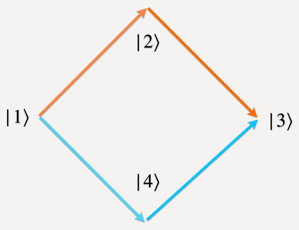
Diagram of two routes from state |1⟩ to state |3⟩: an upper orange path through intermediate state |2⟩ and a lower blue path through intermediate state |4⟩. — **Figure 1.** Schematic diagram depicting a transition from |1⟩ to |3⟩ via two different routes respectively with intermediate state |2⟩ and |4⟩.

Geometric phase in quantum interference phenomenon

Suppose we are given a non-relativistic quantum system which is initially prepared in a normalised state $|1\rangle$ . We are told that it can transition to the final normalised state $|3\rangle$ via two mutually exclusive routes as shown in Figure 1. Firstly it can transition to $|2\rangle$ and then to $|3\rangle$ : $|1\rangle \rightarrow |2\rangle \rightarrow |3\rangle$ . Or secondly it can transition to $|4\rangle$ and then can go to $|3\rangle$ : $|1\rangle \rightarrow |4\rangle \rightarrow |3\rangle$ . Being mutually exclusive implies that the states $|1\rangle$ and $|3\rangle$ are orthogonal. Actually such a system captures the essence of a large class of quantum interference phenomena [16]. As per the Feynman’s second general principle of quantum mechanics [3], the total transition amplitude $A_{1234}$ for such a process is the sum of the amplitudes along both the routes:

Evidently the probability of this transition would display an interference effect, owing to the relative phase difference: $\text{Arg}\,\langle 1|2\rangle\langle 2|3\rangle - \text{Arg}\,\langle 1|4\rangle\langle 4|3\rangle \equiv \text{Arg}\,\langle 1|2\rangle\langle 2|3\rangle\langle 3|4\rangle\langle 4|1\rangle$ between the two superposed amplitudes. Explicitly it reads:

P_{1234} = |⟨1|2⟩⟨2|3⟩|^2 + |⟨1|4⟩⟨4|3⟩|^2 + 2|\Delta_{1234}| cos(Arg \Delta_{1234}) (6)

where $\Delta_{1234} = \langle 1|2\rangle\langle 2|3\rangle\langle 3|4\rangle\langle 4|1\rangle$ is the Bargmann invariant that governs the interference phenomenon. It is remarkable to note that the interference extrema are due to the geometric phase $\gamma_{1234} = \text{Arg}\,\Delta_{1234}$ .

It is worth emphasizing that the presence of geometric phase in such a simple and basic interference problem, which is central to many quantum phenomena, has not been noticed earlier.

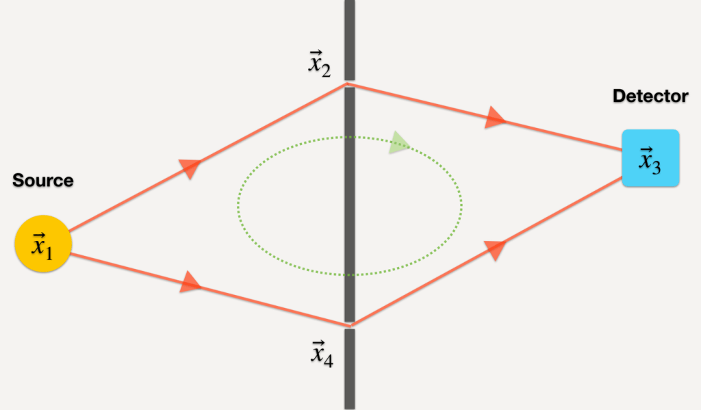
Young's double slit setup: a source at x1 sends paths through slits at x2 and x4 in a barrier to a detector at x3, with a dotted loop around the barrier marking the integration path. — **Figure 2.** Depiction of Young’s double slit experiment. The dotted line represents the path of integration.

Geometric phase in double slit experiment

Above interference phenomenon reminds one of the classic Young’s double slit interference experiment [3] as shown in Figure 2. Here the initial state of the particle is $|\vec{x}_{1},t_{1}\rangle$ which represents a sharply localised normalised state at position $\vec{x}_{1}$ at initial time $t_1$ , while $|\vec{x}_{3},t_{3}\rangle$ represents the same at $\vec{x}_{3}$ and at final time $t_3$ when the particle reaches the detector. It is allowed to pass through the two infinitesimally narrow slits located respectively at $\vec{x}_{2}$ and $\vec{x}_{4}$ . The transition amplitude for such a process is:

T = ⟨x1,t1|x2,t2⟩⟨x2,t2|x3,t3⟩ + ⟨x1,t1|x4,t4⟩⟨x4,t4|x3,t3⟩ (7)

where we have assumed that the particle reaches the first slit at time $t_2$ and the second slit at time $t_4$ respectively. Interestingly the transition amplitude $\langle\vec{x}_{i},t_{i}|\vec{x}_{j},t_{j}\rangle$ is the well known Feynman propagator [17, 18] which is expressible as a path integral:

⟨x_i,t_i|x_f,t_f⟩ = \int Dx e^{iS[x]/\hbar} (8)

where the action $S[\vec{x}] = \int_{t_{i}}^{t_f} dt\,\frac{m}{2}\dot{\vec{x}}\cdot\dot{\vec{x}}$ . It is remarkable to note that while each of the paths (amongst the infinitely many) connecting $\vec{x}_{i}$ to $\vec{x}_{f}$ contributes respective phase $e^{\frac{i}{\hbar}S[\vec{x}]}$ to the propagator, upon an exact explicit evaluation the phase contribution only due to the classical path survives [18]:

Free particle propagator = (m / 2\pi i\hbar(t_f - t_i))^{3/2} e^{i m (x_f - x_i)^2 / 2\hbar(t_f - t_i)} = N_{if} e^{iS[x_cl]/\hbar} (9)

Here $\vec{x}_{cl}$ represents the rectilinear classical path $\vec{x}_{cl}(t) = \vec{x}_{i} + \frac{(\vec{x}_{f} - \vec{x}_{i})}{(t_{f} - t_{i})}(t - t_{i})$ . Thus one learns that in quantum mechanics while the particle moving in free space is allowed to take all the possible paths as is usually taught [3], the non-trivial contribution actually only comes from the classical path.

In light of this result, we see that the transition amplitude of the Young’s double slit experiment is expressible as:

T = N_12 N_23 e^{iS_123/\hbar} + N_14 N_43 e^{iS_143/\hbar} (10)

where $S[\vec{x}_{cl}]_{123}$ stands for the action evaluated along the classical paths connecting $\vec{x}_{1}$ to $\vec{x}_{2}$ and $\vec{x}_{2}$ to $\vec{x}_{3}$ , and respectively for $S[\vec{x}_{cl}]_{143}$ . This tells us that the phase difference between the two amplitudes that gives rise to the interference is the geometric phase $\gamma$ :

\gamma = (S_123 - S_143)/\hbar = \frac{1}{2\hbar}\oint_{1234} \vec p\cdot d\vec x (11)

The integration here is meant to be performed along the quadrilateral formed by vertices $\vec{x}_{j}$ ( $j=1,2,3,4$ ) in the order $1 \rightarrow 2 \rightarrow 3 \rightarrow 4 \rightarrow 1$ .

This result essentially establishes the connection of Young’s double slit interference phenomenon with the notion of geometric phase.

In the case, when the two slits are equidistant from the source, and when the separation between the slits $d$ is much smaller than the distance between the slits and the detector, (11) simplifies considerably to read [19]:

\gamma = \frac{2\pi d}{\lambda} \sin\theta (12)

where $\lambda$ is the corresponding de-Broglie wavelength whereas $\theta$ is the angle formed between the line normal to the slit and the detector. From (6) it is clear that the maxima occur when $\gamma = 2\pi n$ , ( $n$ being integer), which readily provides us with the familiar maxima condition: $n\lambda = d\sin\theta$ [1].

In the above discussion we have dealt with the interference phenomenon of a non-relativistic point particle, and one might wonder about the existence of geometric phase, as discovered above, in the optical case as well. It is well known from the landmark work of Fermat that the optical propagation can indeed be cast into a classical mechanical framework wherein the optical pathlength $\mathcal{S} = \int_{\vec{x}_i}^{\vec{x}_f} ds$ between points $\vec{x}_{i}$ and $\vec{x}_{f}$ plays the role of action, where $ds = \sqrt{d\vec{x}\cdot d\vec{x}}$ [1, 20]. Light takes all possible paths between the two points, while the shortest distance path which extremises the action yields the geometrical optics limit. The geometrical optics limit, in which case $\lambda \rightarrow 0$ is considered, is conceptually same as the semiclassical limit for a point particle system, wherein $h \rightarrow 0$ [21, 22]. In this light, the geometric phase for the optical version of the double slit experiment essentially is:

\Gamma = \frac{2\pi}{\lambda}(S^{geo}_123 - S^{geo}_143) = \frac{2\pi}{\lambda}\oint_{1234} ds (13)

Here the action is evaluated along the shortest distance path or the geometrical optics path. In case when the slit distance $d$ is small compared to the distance between the slits and the detector, and when the source is equidistant from the slits, one straightaway finds that $\Gamma = \frac{2\pi}{\lambda}(L_{1} - L_{2}) = \frac{2\pi d}{\lambda}\sin\theta$ , which is in agreement with (12) (here $L_{1,2}$ respectively stand for the distances of the slits from the detector), as well as with the standard treatments [1, 20].

Acknowledgements

VMV acknowledges discussions with late Prof. T. Pradhan on several aspects of this work.

References

M. Born and E. Wolf, Principles of Optics: electromagnetic theory of propagation, interference and diffraction of light (Elsevier, 2013).
P. A. M. Dirac, The principles of quantum mechanics, No. 27 (Oxford University Press, 1981).
R. P. Feynman, R. B. Leighton and M. L. Sands, Lectures on Physics. 3. Quantum mechanics (Narosa Publishing House, 1998).
M. V. Berry, Quantal phase factors accompanying adiabatic changes, Proceedings of the Royal Society of London. A. Mathematical and Physical Sciences 392, 45–57 (1984).
J. Anandan, The geometric phase, Nature 360, 307–313 (1992).
S. Pancharatnam, Generalized theory of interference and its applications, Proceedings of the Indian Academy of Sciences-Section A 44, 398–417 (1956).
R. Bhandari and J. Samuel, Observation of topological phase by use of a laser interferometer, Phys. Rev. Lett. 60, 1211–1213 (1988).
S. Ramaseshan and R. Nityananda, The interference of polarized light as an early example of Berry’s phase, Current Science 55, 1225–1226 (1986).
M. V. Berry, Anticipations of the geometric phase, Physics Today 43, 34–40 (1990).
A. Shapere and F. Wilczek, Geometric phases in Physics, Vol. 5 (World Scientific, 1989).
N. Mukunda and R. Simon, Quantum kinematic approach to the geometric phase. I. General formalism, Ann. Phys. (N.Y.) 228, 205–268 (1993).
J. Samuel and R. Bhandari, General setting for Berry’s phase, Phys. Rev. Lett. 60, 2339–2342 (1988).
N. Mukunda, Arvind, E. Ercolessi, G. Marmo, G. Morandi and R. Simon, Bargmann invariants, null phase curves, and a theory of the geometric phase, Phys. Rev. A 67, 042114 (2003).
C. Lanczos, The variational principles of mechanics (Courier Corporation, 2012).
V. M. Vyas, Generalised geometric phase, Physics Letters A 561, 130973 (2025).
G. S. Agarwal, Quantum Optics (Cambridge University Press, 2013).
R. Feynman and A. R. Hibbs, The path integral formulation of quantum mechanics (McGraw-Hill, New York, 1965).
A. Das, Field theory: a path integral approach, Vol. 83 (World Scientific, 2019).
E. R. Jones, R. A. Bach and H. Batelaan, Path integrals, matter waves, and the double slit, European Journal of Physics 36, 065048 (2015).
G. Esposito, G. Marmo and E. C. G. Sudarshan, From classical to quantum mechanics: an introduction to the formalism, foundations and applications (Cambridge University Press, 2004).
L. S. Schulman, Techniques and applications of path integration (Courier Corporation, 2012).
T. Pradhan, Maxwell’s equations from geometrical optics, Physics Letters A 122, 397–398 (1987).